How to excel with Excel functions (Part 2 in the Excel Series)

Microsoft Excel is a widely used Office tool, popular ever since spreadsheets came into existence. Having eased the monotonous, redundant tasks, MS Excel has slowly crept into our lives and now holds an intrinsic value in our lives. But even though this commonly used tool finds usage in every office, the primary functions which make this spreadsheet special is still mysterious to many. 

In the first part of our series, we discussed a few essential Excel tools you need to be aware of. In this part, we bring to you some other formulae and functions which will help save time as and when you make use of MS Excel. 

Excel Formulae

1. Simple Calculations

Not only is Excel an expert at performing complex calculations, but it also is aware of the importance of simple calculations. So, in case you’re looking forward to performing a simple addition, subtraction, multiplication or division, all you need to do is use the required sign with the values or the cell address. For instance, if you need to add values 5 and 6, stored in A1 and A2, and store its value in A3, you can either write =A1+A2 or directly add the two values 5 and 6 in A3. 

Pro tip: You can also make use of certain formulae like =Average(Cell Range) or =SUM(Cell Range) in case you want to calculate the average or the sum of a specific range of cells. 

2. Formulae for Conditional Formatting

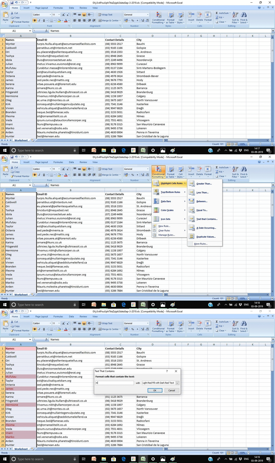
Conditional formatting comes in use when you want to categorize data from different columns and rows on grounds of some commonality. It helps in colour coding the cells based on the information they contain. For instance, if you want to highlight the cells which have m in their names, conditional formatting can help you do that. 

*Click on the GIF for better clarity.

To apply conditional formatting: 

Step 1: Select the cells you want to add it to 

Step 2: Choose ‘Conditional Formatting’ from the Home menu

Step 3: You can then select the logic you want to apply from the dropdown 

Step 4: Click ‘OK’. 

3. The IF Statement

At times, you'll have to add some value against another set of values in a given list. Adding this manually, especially in cases where the data set is large is a tedious task. Thus, to implement this and avoid manual labour, IF statement comes into the picture. 

To make the picture clearer, refer to the following example:

For instance, you might want to add 1 grace mark against the students who score 32 out of 100, 33 being the passing marks.

Step 1: You can then use the IF statement like: “IF(logical_test, value_if_true, value_if_false)”

Step 2: For this example, you can use: “IF(D2= “32”, “1”, “0”)” and press enter.

*Click on the GIF for better clarity.

4. Dollar Signs

The dollar sign in the Excel formula does not represent the American dollar. It instead is used to set an absolute formula to cells. When a formula in respect to specific cells is used (For eg: A5+C5), it gets changed when copied to another cell (an adjacent cell or a cell below) according to the next cells in line i.e., if moved a cell below, the cells will change to A6+C6. But in cases where we do not want the formula to change in respect to the cells, we’ll need to make the formula absolute by adding the dollar sign. In the above example, to fix A5 and C5, we’ll write the formula like “$A$5+$C$5”.

Excel Functions

1. The VLOOKUP Function

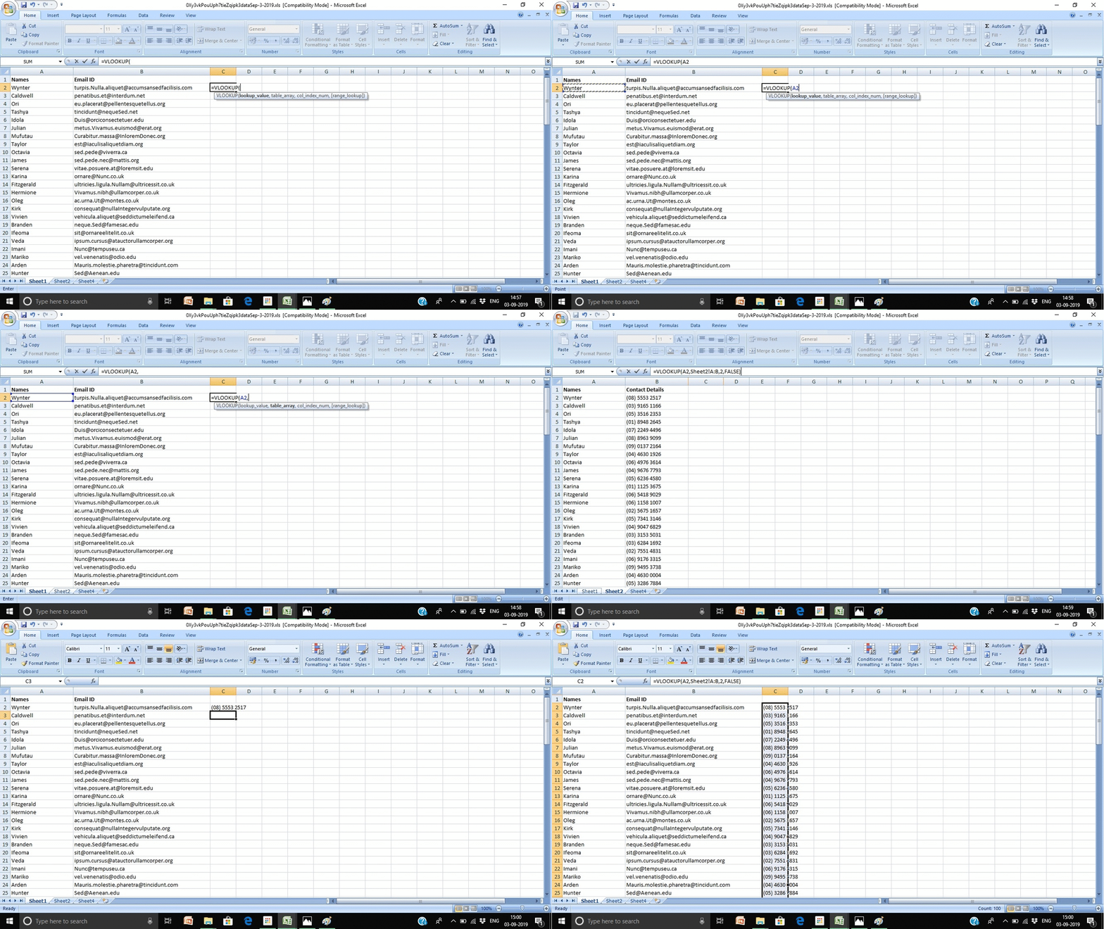
In case you have two Excel sheets having different values and you’d like to merge them, this function can ease your task. For instance, you might have names with their corresponding email IDs in one sheet and names with their contact numbers and addresses in the other, the VLOOKUP function can help you do that easily. However, you need to be sure that you have at least one column that is identical in both the sheets. 

*Click on the GIF for better clarity.

For instance, if you want to merge data from sheet 1 and 2 to sheet 1, with sheet 1 having names and email IDs and sheet 2 having names and contact details, use the following steps:

Step 1: The formula: =VLOOKUP(lookup value, table array, column number, [range lookup])

1. The lookup value is the one that’s identical in both the sheets
2. The table array consists of the range of columns you’re picking from sheet 2 and adding to sheet 1. In our example, this will be “Sheet2!A:B”, where A is the column in sheet 2 which has the data identical to sheet 1. B contains the data which is specific to sheet 2 only
3. Column number indicates the column number of the data in sheet 2 that is to be picked and copied to sheet 1
4. Enter a ‘False’ value in Range lookup, to pick only the exact matches up.

Step 2: For the example we have considered, the formula used will be: =VLOOKUP(C2, Sheet2!A:B, 2, FALSE). After writing then formula, press enter.

VLOOKUP is restricted to picking values up only from the column right next to the column identical to both the sheets. Such limitations make INDEX and MATCH a better option when dealing with Excel functions. 

2. INDEX MATCH

On grounds similar to those of the VLOOKUP function, the INDEX and MATCH function finds usage when data is required to be pulled from a different sheet into a central location. The primary differences between the two formulae are:

1. Where VLOOKUP is a simple formula, INDEX and MATCH comes into play when large data sets with thousands of lookups are in the picture.
2. The VLOOKUP formula works left to right only whereas the INDEX MATCH formula works right to left. This implies that if you have a column in the extreme right of your sheet which you need to look up, you’ll have to rearrange the data in your sheet to use VLOOKUP. This is a tedious process and can lead to errors. 

Let us take an example.

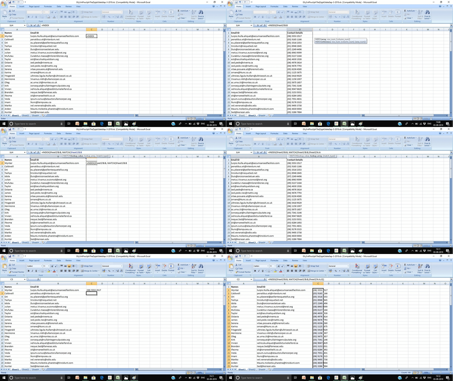
Suppose we have a list of names and their email addresses in sheet 1 and the email addresses and contact numbers in sheet 2. Now, even though we do have a common column in both the sheets, their addresses are different. To use VLOOKUP, we’ll have to rearrange the column in one of the two sheets. So, instead, we make use of the INDEX MATCH function. This, in terms of usage, is similar to VLOOKUP, but forms an integral part of the functions used in Excel. To use INDEX MATCH, follow these steps:

Step 1: The formula: =INDEX(table array, MATCH formula) which is: =INDEX(table array, MATCH (lookup_value, lookup_array))

*Click on the GIF for better clarity.

1. Table array consists of the new data which we need from sheet 2 to be merged in sheet 1. For example, here we need to shift the contact details from sheet 2 (in column B) to sheet 1
2. The lookup value is the address of the column in sheet 1 which is common in both the sheets. Here, for example, the email address is in column B. So, our lookup array will be ‘Sheet1!B:B’
3. The lookup array is the column in sheet 2 which contains values identical to that of sheet 1. If the email addresses from our example are in column A in sheet 2, then our lookup array will be: ‘Sheet2!A:A’.

Step 2: The formula thus used, in the above format, will turn out to be: =INDEX(Sheet2!B:B, (MATCH(Sheet1!B:B, Sheet2!A:A, 0))). Type the formula in the required cell and press enter.

3. The COUNTIF Function

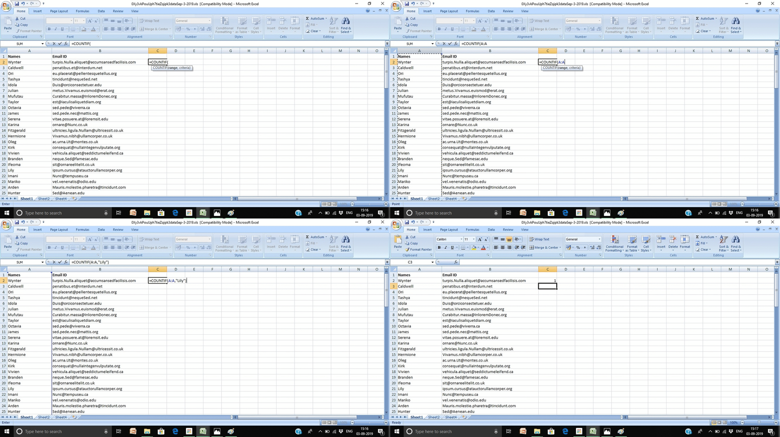
This list of Excel functions will be incomplete without the mention of the COUNTIF function. In places where you need to count the number of times a word or number comes in the sheet, you can use the COUNTIF function instead of counting manually. So, for instance, you need to find how many times the name ‘Lily’ appears in the given data set. Follow these steps:

Step 1:  Use this formula: =COUNTIF(range, criteria)

1. The range indicates the number of columns we are looking in. If we’re looking in two columns C and D, the range will be - C:D
2. The criteria consists of the word/number whose count you desire. In our example, ‘Lily’ is the criteria.

*Click on the GIF for better clarity.

Step 2: The formula thus used will be: =COUNTIF(A:A, “Lily”). After typing the formula, press enter.

4. Using “&” to combine cells

Datasets often split the data out in different columns to make it as appropriate as possible. So, in case a dataset consists of a list of the first name and the last name in different columns, the & function can help you in pulling the entire name out in a single column. 

Suppose you have the first name in column A1 and the last name in column B1 which need to be merged. Follow these steps:

Step 1: Write =A2&“ ”&B2 in the column where the full name is required.

Step 2: Press enter

Step 3: For multiple rows, drag the formula to the entire column.

Note: Ensure that you add space (“ ”) between the two names. This is to differentiate between the first and the last names of the given dataset.  

Having laid our curated pocket list of Excel formulae and functions here, all in one place, we have come to an end of the last part (Part 2) of our Excel series. Decrease your workload by making frequent and better use of Excel in your daily lives. 

With MS Excel is here to your rescue, stop worrying, start working!