Graph Data Structure | Types, Algorithms & More (+Code Examples)

17 mins read

In the world of computer science, a graph is more than just a visual representation—it's a fundamental data structure that captures relationships between entities. Whether you're mapping social networks, optimizing delivery routes, or modeling web pages for search engines, graphs are essential tools for solving complex, real-world problems.

In this article, we’ll explore the concept of graph data structures, their components, types, and practical uses. Additionally, we’ll understand the implementation techniques and algorithms that bring graphs to life in programming.

What Is A Graph Data Structure?

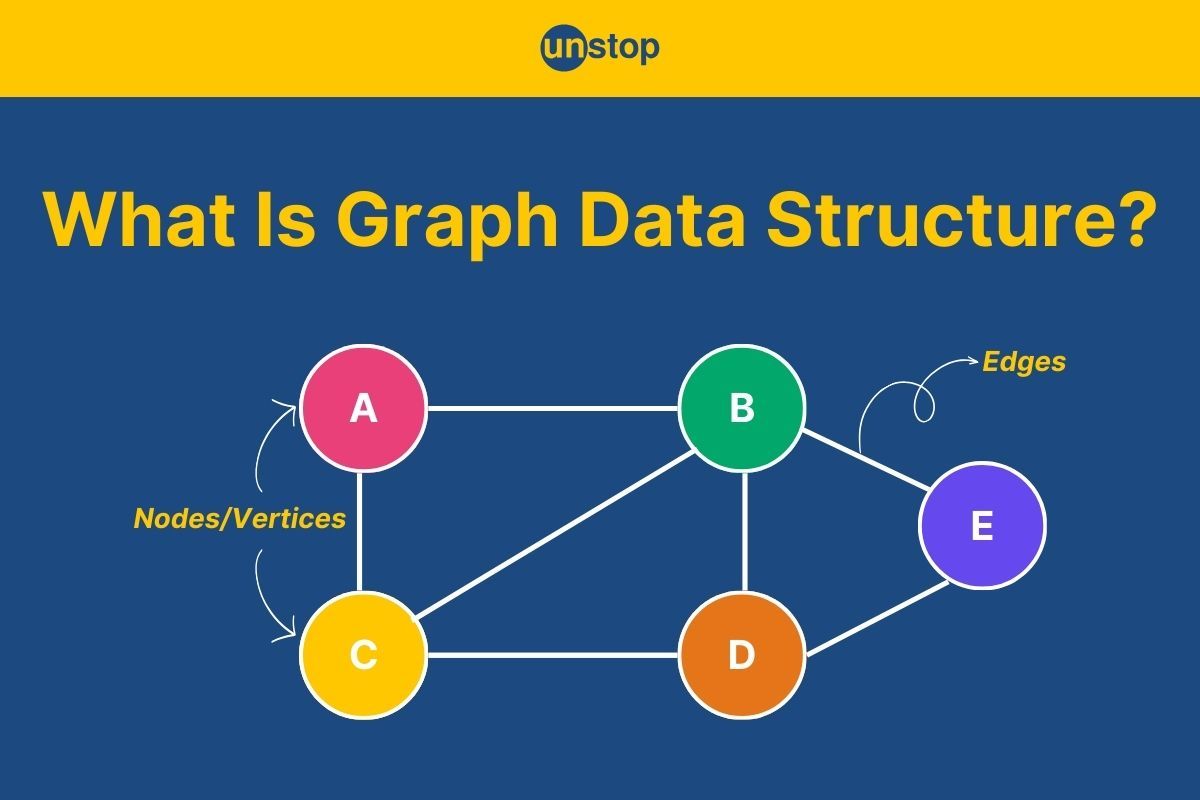
A graph is a mathematical and data structure concept used to represent a set of objects and the relationships between them. It consists of two main components:

1. Vertices (or nodes): These are the individual entities or points in the graph.
2. Edges (or arcs): These are the connections or relationships between the vertices. An edge can be directed (one-way) or undirected (two-way).

In a graph, vertices represent objects, while edges represent the relationships between those objects. This structure can model various real-world systems like social networks, transportation systems, or even computer networks.

Importance Of Graph Data Structures

Graphs are powerful because they can represent complex systems and relationships that are difficult to model using other data structures like arrays or lists. Some key reasons why graphs are important include:

• Versatility: Graphs can model a wide variety of systems, from social networks to transportation routes.
• Dynamic Representation: They allow flexible representation of objects and their relationships, adapting to changes in the real world.
• Efficient Algorithms: Many algorithms for searching, finding the shortest path, and detecting cycles in graphs are highly efficient and widely used in real-world applications.

Types Of Graphs In Data Structure

Graphs can be categorized in various ways based on their structure, directionality, and whether they have additional properties like weights. Below are the most common types of graphs:

1. Directed Graph (Digraph)

• Definition: A directed graph is one in which edges have a specific direction. An edge from vertex A to vertex B is represented as (A → B), meaning the edge points from A to B.
• Key Feature: Each edge has a direction, indicating a one-way relationship.
• Example: A Twitter network where a user follows another user.

2. Undirected Graph

• Definition: In an undirected graph, edges do not have any direction. An edge between vertex A and vertex B is simply represented as {A, B} or (A, B), meaning the relationship is bidirectional.
• Key Feature: Edges represent mutual relationships, where if A is connected to B, B is also connected to A.
• Example: A Facebook friendship network where friendships are mutual.

3. Weighted Graph

• Definition: A weighted graph is a graph in which each edge has a weight or cost associated with it. The weight could represent distance, time, or any other measurable quantity.
• Key Feature: Edges have weights that represent the "cost" or "distance" between vertices.
• Example: A road network where the weight of an edge represents the distance between two cities.

4. Unweighted Graph

• Definition: An unweighted graph is a graph where all edges are treated equally, and no weight is assigned to any edge.
• Key Feature: No weights are associated with edges.
• Example: A simple social network where the edges represent connections but no additional cost or relationship strength is considered.

5. Complete Graph (Kn)

• Definition: A complete graph is one where there is a unique edge between every pair of vertices. In other words, every vertex is connected to every other vertex.
• Key Feature: Every pair of distinct vertices is connected by an edge.
• Example: A fully connected network of people where everyone is connected to everyone else.

6. Bipartite Graph

• Definition: A bipartite graph consists of two sets of vertices, and edges only exist between vertices from different sets, not within a set.
• Key Feature: Vertices can be divided into two disjoint sets, and edges only connect vertices from different sets.
• Example: A job allocation system where one set represents jobs and the other set represents employees, with edges indicating which employee can do which job.

7. Cyclic Graph

• Definition: A cyclic graph is one that contains at least one cycle, which is a path that starts and ends at the same vertex, with no repeated edges or vertices along the way.
• Key Feature: Contains at least one cycle.
• Example: A road system where there’s a circular route connecting cities, allowing for infinite loops.

8. Acyclic Graph

• Definition: An acyclic graph is one that does not contain any cycles. There are no paths that begin and end at the same vertex.
• Key Feature: Contains no cycles.
• Example: A tree structure, such as a family tree, which has no loops.

9. Tree

• Definition: A tree is a special type of acyclic graph that is connected and does not have cycles. It has a hierarchical structure with a single root node, from which all other nodes are descendants.
• Key Feature: Acyclic, connected graph with a hierarchical structure.
• Example: A file system directory structure where each folder contains files or other folders.

10. Forest

• Definition: A forest is a disjoint collection of trees. It can be seen as a set of disconnected trees, each being an acyclic graph.
• Key Feature: A collection of trees (multiple disconnected components).
• Example: A set of independent organizational charts within different departments of a company.

11. Planar Graph

• Definition: A planar graph is one that can be drawn on a plane without any of its edges crossing.
• Key Feature: Can be drawn on a plane without edge intersections.
• Example: A map of cities where each road is represented as an edge, and no two roads cross each other.

12. Sparse and Dense Graphs

• Sparse Graph:
• Definition: A sparse graph has relatively few edges compared to the number of vertices. The number of edges is much smaller than the maximum possible number of edges.
• Example: A graph representing a social network with a small number of connections.
• Dense Graph:
• Definition: A dense graph has a large number of edges, close to the maximum possible edges.
• Example: A fully connected graph, like a social network where most users are friends with each other.

13. Directed Acyclic Graph (DAG)

• Definition: A directed acyclic graph (DAG) is a directed graph that contains no cycles. It is often used in scenarios where the graph represents a flow or process, such as task scheduling.
• Key Feature: Directed edges with no cycles.
• Example: A project dependency graph where tasks are connected by dependencies, and tasks must be completed in a specific order.

14. Multi-Graph

• Definition: A multi-graph allows multiple edges between two vertices. These multiple edges are often called parallel edges.
• Key Feature: Multiple edges between the same pair of vertices are allowed.
• Example: A transportation network where multiple routes connect two cities.

Types Of Graph Algorithms

Graph algorithms are used to solve various problems related to graphs, such as finding the shortest path between vertices, finding minimum spanning trees, and detecting negative weight cycles. Below are some of the most common graph algorithms:

1. Dijkstra’s Algorithm (Shortest Path)

Dijkstra's algorithm is used to find the shortest path from a source vertex to all other vertices in a weighted graph with non-negative edge weights.

Algorithm Steps:

• Initialize the distance to the source vertex as 0 and all other vertices as infinity.
• Visit all vertices, and for each vertex, update the shortest distance using the current vertex’s distance and edge weights.
• Repeat until all vertices are visited.

Code Example:

#include <iostream>
#include <vector>
#include <set>
#include <climits>

using namespace std;

void dijkstra(int V, vector<vector<pair<int, int>>>& adj, int source) {
    vector<int> dist(V, INT_MAX);
    dist[source] = 0;

    set<pair<int, int>> s; // {distance, vertex}
    s.insert({0, source});

    while (!s.empty()) {
        int u = s.begin()->second;
        s.erase(s.begin());

        // Visit all adjacent vertices of u
        for (auto neighbor : adj[u]) {
            int v = neighbor.first;
            int weight = neighbor.second;

            if (dist[u] + weight < dist[v]) {
                if (dist[v] != INT_MAX)
                    s.erase(s.find({dist[v], v}));

                dist[v] = dist[u] + weight;
                s.insert({dist[v], v});
            }
        }
    }

    // Print shortest distances
    for (int i = 0; i < V; ++i) {
        cout << "Distance from " << source << " to " << i << " is " << dist[i] << endl;
    }
}

int main() {
    int V = 5; // Number of vertices
    vector<vector<pair<int, int>>> adj(V);

    adj[0].push_back({1, 10});
    adj[0].push_back({4, 5});
    adj[1].push_back({2, 1});
    adj[2].push_back({3, 4});
    adj[3].push_back({0, 7});
    adj[4].push_back({1, 3});
    adj[4].push_back({2, 9});

    dijkstra(V, adj, 0);

    return 0;
}

Output:

Distance from 0 to 0 is 0
Distance from 0 to 1 is 8
Distance from 0 to 2 is 9
Distance from 0 to 3 is 13
Distance from 0 to 4 is 5

Explanation: 

In this code, we implement Dijkstra's algorithm to find the shortest paths from a source vertex to all other vertices in a weighted graph.

1. Initialization:
• We create a dist vector initialized with INT_MAX to represent infinite distances. The distance from the source to itself is set to 0.
• A set is used to store vertices, prioritizing those with the smallest known distance (pair of distance and vertex).
2. Main Algorithm:
• We repeatedly pick the vertex with the smallest distance from the set (u), then remove it.
• We visit each neighbor of u. If the distance through u to a neighbor v is shorter than the current distance to v, we update it and insert the new distance into the set.
3. Output:
• After the algorithm completes, we print the shortest distance from the source to each vertex.

​​In the main() function, we define a graph with 5 vertices and their respective weighted edges. We then call the dijkstra() function to find and print the shortest distances from vertex 0.

2. Bellman-Ford Algorithm

The Bellman-Ford algorithm can be used to find the shortest path from a source vertex to all other vertices in a weighted graph, including graphs with negative edge weights. It can also detect negative weight cycles.

Algorithm Steps:

• Initialize the distance to the source vertex as 0 and all others as infinity.
• Relax all edges V-1 times, where V is the number of vertices.
• Check for negative weight cycles by relaxing all edges one more time.

Code Example:

#include <iostream>
#include <vector>
#include <climits>

using namespace std;

void bellmanFord(int V, vector<vector<int>>& edges, int source) {
    vector<int> dist(V, INT_MAX);
    dist[source] = 0;

    // Relax all edges V-1 times
    for (int i = 1; i < V; ++i) {
        for (auto edge : edges) {
            int u = edge[0], v = edge[1], weight = edge[2];
            if (dist[u] != INT_MAX && dist[u] + weight < dist[v]) {
                dist[v] = dist[u] + weight;
            }
        }
    }

    // Check for negative weight cycles
    for (auto edge : edges) {
        int u = edge[0], v = edge[1], weight = edge[2];
        if (dist[u] != INT_MAX && dist[u] + weight < dist[v]) {
            cout << "Graph contains a negative weight cycle" << endl;
            return;
        }
    }

    // Print shortest distances
    for (int i = 0; i < V; ++i) {
        cout << "Distance from " << source << " to " << i << " is " << dist[i] << endl;
    }
}

int main() {
    int V = 5; // Number of vertices
    vector<vector<int>> edges = {
        {0, 1, -1}, {0, 2, 4}, {1, 2, 3}, {1, 3, 2}, {1, 4, 2},
        {3, 2, 5}, {3, 1, 1}, {4, 3, -3}
    };

    bellmanFord(V, edges, 0);
    return 0;
}

Output:

Distance from 0 to 0 is 0
Distance from 0 to 1 is -1
Distance from 0 to 2 is 2
Distance from 0 to 3 is -2
Distance from 0 to 4 is 1

Explanation:

In this code, we implement the Bellman-Ford algorithm to find the shortest paths from a source vertex to all other vertices in a graph, while also detecting negative weight cycles.

1. Initialization:
• We create a dist vector, initialized to INT_MAX, to represent infinite distances. The distance from the source to itself is set to 0.
2. Relaxation:
• We relax all edges V-1 times (where V is the number of vertices). For each edge (u, v) with weight w, if the distance to v through u is shorter than the current distance to v, we update the distance to v.
3. Negative Weight Cycle Detection:
• After relaxing all edges, we check each edge again to see if we can further reduce the distance to any vertex. If so, it indicates the presence of a negative weight cycle in the graph.
4. Output:
• Finally, we print the shortest distances from the source vertex to all other vertices. If a negative weight cycle is detected, a message is printed indicating its presence.

In the main() function, we define a graph with 5 vertices and the respective weighted edges. We then call the bellmanFord() function to find and print the shortest distances from vertex 0, or detect a negative weight cycle if one exists.

3. Floyd-Warshall Algorithm

The Floyd-Warshall algorithm computes the shortest paths between all pairs of vertices in a weighted graph. It can handle negative weights but cannot detect negative weight cycles.

Algorithm Steps:

• Initialize a matrix to represent the graph's distances.
• For each vertex, update the shortest distance between every pair of vertices through intermediate vertices.

Code Example:

#include <iostream>
#include <vector>
#include <climits>

using namespace std;

void floydWarshall(int V, vector<vector<int>>& graph) {
    vector<vector<int>> dist = graph;

    // Main algorithm
    for (int k = 0; k < V; ++k) {
        for (int i = 0; i < V; ++i) {
            for (int j = 0; j < V; ++j) {
                if (dist[i][k] != INT_MAX && dist[k][j] != INT_MAX &&
                    dist[i][k] + dist[k][j] < dist[i][j]) {
                    dist[i][j] = dist[i][k] + dist[k][j];
                }
            }
        }
    }

    // Print shortest distances
    for (int i = 0; i < V; ++i) {
        for (int j = 0; j < V; ++j) {
            if (dist[i][j] == INT_MAX)
                cout << "INF ";
            else
                cout << dist[i][j] << " ";
        }
        cout << endl;
    }
}

int main() {
    int V = 4;
    vector<vector<int>> graph = {
        {0, 3, INT_MAX, INT_MAX},
        {2, 0, INT_MAX, 4},
        {INT_MAX, 7, 0, 1},
        {INT_MAX, INT_MAX, 2, 0}
    };

    floydWarshall(V, graph);
    return 0;
}

Output:

0 3 9 7
2 0 6 4
9 7 0 1
11 9 2 0 

Explanation:

In this code, we implement the Floyd-Warshall algorithm to find the shortest paths between all pairs of vertices in a weighted graph.

1. Initialization:
• We create a dist matrix that initially holds the input graph, where dist[i][j] represents the distance from vertex i to vertex j. If no direct edge exists between two vertices, the distance is set to INT_MAX (infinity).
2. Main Algorithm:
• The algorithm iterates through each possible intermediate vertex k and tries to improve the distance between every pair of vertices (i, j) by checking if the path from i to j through k is shorter than the current known distance. If it is, the distance is updated.
3. Output:
• After completing the algorithm, we print the shortest distances between every pair of vertices. If the distance is INT_MAX, it is printed as "INF" to indicate no path exists between the vertices.

In the main() function, we define a graph with 4 vertices and the respective edge weights. We then call the floydWarshall() function to compute and print the shortest distances between all pairs of vertices.

4. Kruskal’s Algorithm (Minimum Spanning Tree)

Kruskal's algorithm finds the minimum spanning tree (MST) of a graph by adding edges in increasing order of weight, ensuring no cycles are formed.

Algorithm Steps:

• Sort all the edges in non-decreasing order of weight.
• Add edges one by one to the MST, using a union-find data structure to detect and avoid cycles.

Code Example:

#include <iostream>
#include <vector>
#include <algorithm>

using namespace std;

struct Edge {
    int u, v, weight;
    bool operator<(const Edge& e) const {
        return weight < e.weight;
    }
};

int find(int parent[], int x) {
    if (parent[x] == x)
        return x;
    return parent[x] = find(parent, parent[x]);
}

void unionSet(int parent[], int rank[], int x, int y) {
    int rootX = find(parent, x);
    int rootY = find(parent, y);

    if (rootX != rootY) {
        if (rank[rootX] > rank[rootY])
            parent[rootY] = rootX;
        else if (rank[rootX] < rank[rootY])
            parent[rootX] = rootY;
        else {
            parent[rootY] = rootX;
            rank[rootX]++;
        }
    }
}

void kruskal(int V, vector<Edge>& edges) {
    sort(edges.begin(), edges.end());
    int parent[V], rank[V];
    for (int i = 0; i < V; ++i) {
        parent[i] = i;
        rank[i] = 0;
    }

    vector<Edge> mst;
    for (Edge e : edges) {
        int u = e.u, v = e.v;
        if (find(parent, u) != find(parent, v)) {
            mst.push_back(e);
            unionSet(parent, rank, u, v);
        }
    }

    // Print MST edges
    for (Edge e : mst) {
        cout << e.u << " - " << e.v << " : " << e.weight << endl;
    }
}

int main() {
    int V = 4;
    vector<Edge> edges = {{0, 1, 10}, {0, 2, 6}, {0, 3, 5}, {1, 3, 15}, {2, 3, 4}};

    kruskal(V, edges);
    return 0;
}

Output:

2 - 3 : 4
0 - 3 : 5
0 - 1 : 10

Explanation:

In this code, we implement Kruskal's algorithm to find the Minimum Spanning Tree (MST) of a graph.

1. Edge Structure:
• We define an Edge struct to store the vertices (u, v) and the weight of the edge between them. We also define an overload for the < operator to sort edges by their weights.
2. Find and Union Operations:
• The find() function uses path compression to find the root of a given vertex, ensuring efficient operations for disjoint sets.
• The unionSet() function unites two sets containing vertices x and y based on their ranks. The rank is used to keep the tree flat during the union process, optimizing the find operation.
3. Main Algorithm:
• In the kruskal() function, we first sort the edges in increasing order of weight.
• We initialize two arrays: parent[] to store the representative of each vertex and rank[] to store the rank of each vertex for union operations.
• We then iterate over the edges, adding an edge to the MST if it connects two different sets (i.e., no cycle is formed). We use the find() and unionSet() functions to manage the disjoint sets.
4. Output:
• Finally, we print the edges of the MST along with their weights.

In the main() function, we define a graph with 4 vertices and the respective edges with weights. We then call the kruskal() function to find and print the edges of the MST.

Application Of Graphs In Data Structures

Graphs are used in many fields due to their ability to model relationships between entities. Some examples include:

1. Social Networks: In platforms like Facebook or Twitter, users are represented as vertices, and their connections (friends, followers) are represented as edges.
2. Navigation Systems: Graphs represent cities or locations as vertices and the roads between them as edges. This structure is essential for GPS and map applications, especially when finding the shortest path between two locations.
3. Computer Networks: In networking, computers or devices are vertices, and communication channels (like routers and switches) are edges. This helps in routing data efficiently.
4. Recommendation Systems: Websites like Amazon or Netflix use graph structures to recommend products or movies by analyzing the relationships between products, users, and preferences.
5. Web Crawling: The web itself can be viewed as a graph, where web pages are nodes and hyperlinks between them are edges. Graph algorithms help web crawlers index pages efficiently.

Challenges And Complexities In Graphs

Graphs, despite their versatility and wide applications, present several challenges in both theoretical and practical contexts. Here are some key challenges and complexities associated with graphs:

1. Scalability:

• • As the number of vertices and edges in a graph increases, the space and time complexity of operations can become very large.
  • Algorithms like Dijkstra’s, Bellman-Ford, or Floyd-Warshall require efficient handling of large graphs to avoid performance degradation.
  • Sparse graphs (with fewer edges) may require different approaches compared to dense graphs (with many edges), as dense graphs tend to have higher time complexities due to the large number of edges.

2. Memory Consumption:

• • Storing large graphs can be memory-intensive, especially when using adjacency matrices for dense graphs. Adjacency lists are more memory-efficient for sparse graphs but may still require significant space for very large graphs.
  • For instance, an adjacency matrix requires O(V^2) space (where V is the number of vertices), whereas an adjacency list uses O(E) space (where E is the number of edges).

3. Cycle Detection:

• • Detecting cycles in graphs is crucial for ensuring data consistency, especially in directed graphs or when dealing with feedback loops.
  • Algorithms for cycle detection (like DFS-based approaches) may face challenges with graphs that have many complex interactions, leading to high computational costs.

4. Negative Weight Cycles:

• • In the presence of negative weight edges, algorithms like Dijkstra’s algorithm fail to give correct results, requiring us to use alternatives like Bellman-Ford or modifications for accurate handling.
  • Additionally, detecting negative weight cycles can complicate algorithms and extend their running time, as we need to repeatedly check for updates after each iteration.

5. Graph Traversal:

• • Traversing large or complex graphs efficiently, whether through BFS (Breadth-First Search) or DFS (Depth-First Search), can become a challenge if the graph is unbalanced or contains deeply nested structures.
  • Recursive depth-first searches can lead to stack overflow errors when dealing with deep or large graphs unless iterative methods are employed.

6. Shortest Path Problem in Dynamic Graphs:

• • In real-world applications, graphs are often dynamic (edges and vertices can change over time). Updating shortest paths when the graph is modified can be a difficult challenge.
  • Algorithms such as Dijkstra’s or Bellman-Ford need to be adapted for dynamic graphs to handle frequent updates efficiently.

7. Graph Coloring and NP-Completeness:

• • Problems like graph coloring, where vertices are assigned colors such that no two adjacent vertices share the same color, are NP-complete in the general case.
  • These types of problems require heuristic or approximation algorithms to find acceptable solutions in practical scenarios.

8. Edge Weights and Heuristics:

• • Graph algorithms that involve weighted edges (like the shortest path algorithms) may be sensitive to the way edge weights are assigned. Poorly chosen weights or heuristics can lead to suboptimal or incorrect results, especially in algorithms like A* that rely on heuristic functions.

9. Parallelism and Distributed Graph Processing:

• • Efficiently processing large graphs in parallel or in a distributed manner remains a challenge. Issues like load balancing, synchronization, and handling distributed data become significant obstacles when working with massive-scale graphs, such as social networks or large-scale recommendation systems.

10. Handling Infinite Graphs:

• • In certain applications (e.g., navigation, AI), we may encounter graphs that are theoretically infinite or unbounded. Handling such graphs, where all possible paths are not known upfront, requires specialized techniques like approximations or online algorithms.

Complexity Of Graph Algorithms:

• Time Complexity: The time complexity of graph algorithms can vary significantly. For example:
• Dijkstra’s algorithm with a priority queue runs in O(E log V).
• Bellman-Ford runs in O(VE).
• Floyd-Warshall runs in O(V^3).
• Kruskal’s algorithm runs in O(E log E), while Prim’s runs in O(E log V).
• Space Complexity: Storing a graph typically involves storing all vertices and edges, which results in a space complexity of O(V + E). However, this may differ based on the representation (adjacency list vs adjacency matrix).

Conclusion

Graph data structures are powerful tools for modeling relationships in a variety of applications, from social networks to routing algorithms. Understanding their components, types, and how they are represented helps us effectively utilize them in solving complex problems. With the exploration of key graph algorithms and real-world use cases, we can see how versatile and essential graphs are in computer science. As technology advances, the role of graphs will only continue to grow, making it crucial to understand their foundational concepts and applications.

Frequently Asked Questions

Q. What is the difference between a directed and an undirected graph?

A directed graph (or digraph) has edges with a direction, meaning they go from one vertex to another (e.g., one-way streets). An undirected graph, on the other hand, has edges that do not have a direction, indicating mutual relationships (e.g., two-way streets).

Q. What is the purpose of using a weighted graph?

A weighted graph assigns a weight (or cost) to each edge, representing the strength, distance, or any other metric between the connected vertices. This is useful for algorithms like Dijkstra’s for finding the shortest path where the cost of traveling along edges matters.

Q. How do graph traversal algorithms like DFS and BFS work?

Depth-First Search (DFS) explores a graph by going as deep as possible along a branch before backtracking. Breadth-First Search (BFS) explores the graph level by level, visiting all neighbors of a node before moving to the next level. Both algorithms are essential for various graph-related tasks like searching, finding paths, and detecting cycles.

Q. What is a cycle in a graph?

A cycle in a graph occurs when a path starts and ends at the same vertex, without retracing any edge. In directed graphs, cycles are particularly important to detect, as they can lead to issues like infinite loops in algorithms.

Q. What are the main applications of graph data structures?

Graphs are widely used in applications like social networks (modeling user connections), web crawling (tracking links between pages), transportation systems (shortest path finding), recommendation systems (suggesting products based on user preferences), and many more.

Suggested Reads:

1. Difference Between Hashing And Encryption Decoded
2. 53 Frequently Asked Linked List Interview Questions With Answers 2024
3. Data Structure Interview Questions For 2024 [With Detailed Answers]
4. Tree Topology | Advantages & Disadvantages In Computer Network
5. Decoding Data Redundancy In DBMS| Causes, Advantages, Solutions